Gold Standard for BEV Post Processing

Software/tool names have been changed to protect owners’ copyright and trademarks.

As a Battery Electric Vehicle (BEV) Optimization and Analysis Lead at Stellantis, I was responsible for developing future BEVs using simulations while optimizing their electric range, performance, and capabilities depending on consumer demands. While working on new simulation models to compute electric range, there was a regular problem that the team faced. The article walks through that problem. BVERE was created to tackle that problem. However, it grew to encompass other functionality that the global team demanded.

Tech Stack

#

• Version 1:
  • MATLAB
  • MATLAB GUIde - a tool to create graphical user interfaces (GUIs)
• Version 2:
  • Python 3.7
  • Libraries:
    • Data wrangling and analysis: NumPy, SciPy, Matplotlib
    • GUI development: PyQt5
    • Excel writing: OpenPyXL

Background

#

PACE, an internally developed software, was used to run vehicle simulations to compute and optimize electric range. Developed in MATLAB and Simulink, PACE had a Microsoft Excel interface for users to input relevant data for the vehicle. A complex system like a vehicle includes many attributes with different values as well as components with varying efficiency maps and operating limits. The Excel interface allowed users to interact with these complex data inputs efficiently.

PACE was maintained by an internal Development Team who seldom worked on simulating actual vehicles. They shipped the software as an executable and .dlls to Analysis Engineers who then developed PACE vehicle models by interacting with the Excel interface. As with most large companies, access to the source code of PACE was limited to the Development Team, and we on the Analysis side were forced to grapple with its deficiencies or raise issues/feature requests.

BVERE was born out of grappling with PACE while still maintaining equilibrium with my best quality: indolence.

(Initial) Problem

#

It all started out with this convoluted and nuanced problem.

Electric Range Background

#

When a new battery electric vehicle is developed, it needs to go through regulatory certifications through varied government agencies. One such certification is with the Environmental Protection Agency (EPA) for the vehicle’s electric range. A vehicle’s electric range is displayed, among other things, on the “window” sticker for a particular specification. The idea is for consumers to quickly and easily compare electric ranges of different vehicles when they walk into dealerships for making informed decisions. In today’s world, people don’t visit multiple dealerships in a day; they first research online. The EPA maintains fueleconomy.gov where a consumer can get the electric range (and fuel economy) values for any vehicle sold in the US. You can also compare multiple vehicles from different manufacturers, like I did here.

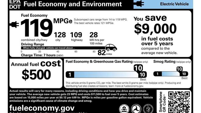
To ensure a fair comparison for passenger electric vehicles, EPA defines standardized driving profiles that every manufacturer has to test their vehicle against. EPA also provides formulas where the manufacturer inputs key data to compute the window sticker electric range. In the picture above, the electric range is 82 miles.

Drive Profiles

#

The Society of Automotive Engineers (SAE) provides numerous standards and procedures to test different aspects of vehicles. EPA uses multiple SAE standards to define BEV certification procedures, especially the drive profiles used for calculating sticker electric range. SAE standard J1634 - Battery Electric Vehicle Energy Consumption and Range Test Procedure - defines these drive profiles for modern BEVs.

The 2017 update to SAE J1634 defined a Multi-Cycle Test (MCT) to determine electric range for BEVs. As modern BEVs have significantly high electric range and manufacturers want to minimize usage of test facilities, the MCT is a quick test (~4-6 hours or one working shift) that represents typical US driving and is designed to test the full spectrum of battery state of charge (SOC).

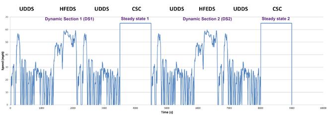
The MCT has four sections and majority of these parts are repeated at high and low vehicle SOCs. Dynamic section 1 (DS1) and dynamic section 2 (DS2) are the same where DS2 is run at a lower SOC. Steady state 1 (SS1) exists to rapidly deplete the battery by running a constant 65MPH to get to ~25% SOC. Steady state 2 (SS2) achieves the same purpose and is designed to completely drain the battery, till the vehicle cannot maintain 65MPH for 10 seconds. Running a vehicle from the highest SOC to the lowest provides the total energy storage capacity of the installed battery pack, which is later used in calculations to determine electric range.

The dynamic sections are divided into two UDDS and one HFEDS parts.

Urban Dynamometer Driving Schedule (UDDS)

#

The MCT contains four UDDS sections - two in both high and low SOC regions. These are what the EPA calls “city” driving, where you have multiple stops due to traffic lights or stop signs or actual traffic. With an average speed of about 30 MPH, it accurately represents majority of the city driving across the country. Of course, there are outliers like New York or Chicago or Los Angeles at peak traffic times.

Highway Fuel Economy Driving Schedule (HFEDS or HWY)

#

Highway driving schedule represents rural highway driving. These are mostly 55 MPH speed limit roads. This does not represent freeway driving at 65 MPH to 75 MPH, where people sometimes drive 85 MPH (guilty ). There are two HFEDS sections in the MCT, one in each high and low SOC regions.

Back to PACE

#

PACE required its users to input two key parameters to run simulations: the drive profile as a speed and time column, and a start SOC value. This was the main problem to effectively simulate the full MCT. More specifically, while making the drive profile, how much time should be allocated to the steady state 1 (SS1) portion so that the dynamic section 2 starts at around 25% SOC. As it turns out, back-calculating this for a vehicle is very hard; I tried. Component operation changes when things gradually heat up in a vehicle, and accounting for all these nuances for all components is time consuming. There is also interdependence between components and attributes, where one might affects other’s operation at any given time. Furthermore, doing this for each simulation for tens of vehicles exasperates the problem. Therefore, determining a drive profile (speed versus time) for each simulation was daunting and the process, even if developed, would be frail as we could easily miss edge cases.

Even if a drive profile were developed for a particular vehicle using the strenuous back-calculating method, the nature of our team’s work would render its use ineffective for the next simulation. Here is a typical scenario that I would encounter at Stellantis: can you change the motor map from supplier X to supplier Y on the New Fiat 500 BEV to determine its impact on range? Also, we are looking at some tire and aerodynamic improvements, give us an impact of electric range for those factors as well. Now, even if we had the drive profile for the base Fiat 500 BEV, changing the motor map would imply creating a new one due to component nuances I touched on earlier. And so would changing tires and aero attributes. What if they wanted all the changes together, that’s a fourth drive profile; keeping up with all these individual files would be harder than keeping up with the Kardashians.

Moreover, specific signals from the simulations were inputted into the calculator provided by EPA to compute electric range. These signals were to be extracted for all parts of the MCT, accurately. A slight mismatch of starting SOC in any of the parts could be a difference between a 250-mile vehicle to a 230-mile vehicle, a deficit so large that several VPs would be involved in discussions (crisis meetings, is what we called them).

Fetch and Fix (part of BVERE)

#

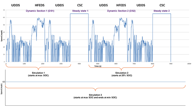
The problem was manageable when I made it about post processing. Rather than running one simulation with the perfectly formed drive cycle (which was impossible without significant trial and error), I ran three simulations. Running three simulations is quicker than the trial and error involved with getting the elusive drive profile right.

The three simulations are enumerated below. They take a total of about 5-6 minutes to complete, depending on the charge a battery pack could hold.

1. Dynamic section 1 run from the highest SOC
2. Dynamic section 2 run from 25% SOC
3. Running a steady state simulation at 65 MPH from the highest SOC to the lowest SOC where the vehicle could not maintain its speed for 10 seconds

With these three simulations, I had all the pieces required to post process their outputs and calculate range for a simulation.

Post Processing Outputs

#

The beginning of Fetch and Fix’s responsibilities involved post processing the outputs of the three simulations, and it contained multiple steps. First of all, end SOC values of Simulations 1 and 2 (dynamic section simulations) were noted. Second, these SOC values were then used to cut the Simulation 3 output (steady state test) into two places. Third, a final cut was made to the steady state output at 25% SOC or wherever Simulation 2 began. Fourth, output from Simulation 1, Simulation 2 and the remainder pieces of the steady state simulation were merged to form a complete MCT drive profile.

As we did this with simulation outputs, all of the data from the simulations was merged (data of motor, inverter, battery, gearbox, etc.) into one large dataset. This data could now be used to calculate electric range for that configuration.

Calculating Range

#

The next responsibility for Fetch and Fix was to calculate key energy and distance metrics for sub-sections of the MCT, and output them them into an Excel calculator. The Excel calculator was configured as per SAE J1634 formulas. The calculator expected energy expenditure in \(Wh\) and distance in \(miles\) for all MCT’s subsections, namely: UDDS1, UDDS2, UDDS3, UDDS4, HWY1, HWY2, SS1 and SS2.

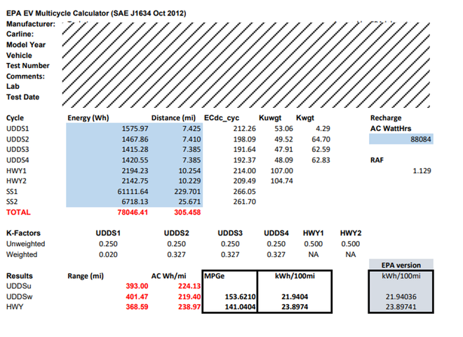
With these inputs, the calculator computed the unadjusted values for the city and highway electric range (represented by UDDSw of 401.47 miles and HWY of 368.59 miles). These values were then multiplied by a factor of \(0.7\), to get the adjusted range. The adjusted range was used to calculate the combined electric range - displayed on the window sticker - using a weighted average. The weights used were 0.55 for UDDS and 0.45 for HFEDS to represent most people’s everyday drives which includes 55% of city driving and 45% of highway driving.

For detailed formulas and some pseudo-code, check out the Appendix of this article at the bottom.

Other Tooling in BVERE

#

When I first started the tool in 2020, it started out with a command line interface (CLI) and only had Fetch and Fix. However, as the tool proliferated beyond me, where other engineers started using it, I started adding more features to it. This is where two other, very talented engineers (FD and DM) got involved in the development of BVERE.

Energy balance

#

According to the law of conservation of energy, the summation of energy expenditures should equal the energy from the source. An energy balance provides an accounting of all the energy expenditures for a particular simulation. These are useful in comparing simulations and understand how a certain component or attribute affected the energy expenditure on a drive profile. For example, if the weight increased by 500 lbs., you would not just expect a change in energy consumption from vehicle demand. There could be upstream effects as well: for instance, increased weight may force the motor to operate in an inefficient area of its operating map, changing it’s energy fingerprint, cumulatively making the system worse. An energy balance clearly highlights these differences.

Bubble Plotter

#

Speaking of motor operation on an operating map. It is helpful to know where the motor is operating for a given drive cycle depending on simulation inputs (attributes and components). Bubble plotter compared two simulations by plotting time-spent based bubbles on motor maps - represented as torque (Nm) versus speed (RPM). The efficiency curves of the motor was the underlay of this plot as a contour (i.e., colored Z-axis in a 2-d plot). The plot, therefore, provided various pieces of information at a glance: how many points from the drive profile were in which regions of the map, and what was the efficiency of the most populous region.

These plots were then used to modify operating strategy/calibrations or communicate to motor subject matter experts of potential improvements to the motors for a certain improvement in electric range. Design of experiment or sweep studies could be performed by changing one factor at a time over a slew of values to identify which parameter caused the operation to be in the most efficient region.

5-Cycle Simulator and Analyzer

#

Remember the \(0.7\) factor in the calculator section before? This factor reduces the “real” or unadjusted electric range to compute adjusted range that would be on the window sticker for all consumers to compare. There is an incentive for manufacturers to display a high electric range number on their stickers. Increasing this factor to greater than 0.7 would mean that the unadjusted range would be penalized less. Running 5-cycles gives a manufacturer the opportunity to increase this factor.

The 5-cycle simulator and analyzer used Python’s multi-threading functionality to simulate 5 cycles in parallel. This functionality also post processed the data from these simulations to compute electric range. The calculations from these 5 cycles to compute electric range are different than the 2-cycle method I have described before, and is a large topic in itself (hopefully, I will cover this in a technical article).

Others

#

There was additional ancillary functionality baked into BVERE.

• Mean energy efficiency and losses calculations
• Vehicle demand energy and powertrain system efficiency calculations
• Vehicle demand energy calculator

These made some ad-hoc request analyses simpler and streamlined. It bolstered trust in the tool and led to wider adoption that may have been limited had these calculators not included.

About Tech Stack Change

#

Version 1 of BVERE was developed in MATLAB. This was an easy choice because the simulation outputs from PACE were MAT files, i.e. MATLAB compatible files. However, as the tool evolved to have more functionality beyond Fetch and Fix, limitations of MATLAB started to emerge. Three key limitations were:

1. MATLAB licensing

   New engineers joining the company were not added to the same MATLAB license pool. Contract hires were not added in any license pool. For them, obtaining a MATLAB license when on company network was like winning a lottery. Moreover, MATLAB licensing was different in Stellantis’ different regions (US, Italy, China and India). This made it very hard for me to ship BVERE to all Analysis Engineers and align them to a common process.

2. MATLAB’s parallel computing inefficiency

   To use parallel computing in MATLAB, you need to purchase a toolbox (bizarre right?). Even when you have the toolbox and want to use it, one has to wait a good minute or two for it to “spool” its parallel workers. Only after all the workers are spooled it will start running the code, i.e. a synchronous task.

3. Lack of unit test functionality

   Although this functionality is added in later MATLAB versions, this was absent in the 2018a version that we were using at Stellantis. This made shipping code without bugs very hard.

I chose Python, selfishly, because that was the (only) other programming language I was able to program in. Plus, it eliminated all of the disadvantages that MATLAB presented. I used pyinstaller to convert the GUI into an executable which engineers could download from a sharepoint. Python’s built in multi-threading and multi-processor functionality made it easy for running simulations in parallel using all cores of the machine, and most importantly by not paying a license fee. Lastly, Python’s built in testing support was easy to use to unit test key calculations and logic pathways to ensure bug-free software.

Moreover, the vast free and open source library ecosystem that Python brought helped us with data analysis, calculations and GUI development. scipy ships with functionality to read MAT files as well, removing that last hurdle of reading MAT simulation output files.

Appendix

#

1. Energy expenditure in Watt-hour (\(Wh\))

Watt-hour is calculated by integrating battery terminal power (in Watts \(W\)) over a drive-cycle section time.

$$E = \int_0^t P.dt$$

With time measured in seconds, captured with a certain frequency for all sections, energy can be calculated in \(Wh\) using trapezoidal integration and multiplying it by the reciprocal of measurement frequency. This provides energy in \(Wsec\). To convert it to \(Wh\), you divide it by 3600.

energy = trapz(power) * (1 / frequency) / 3600

2. Distance traveled (miles)

Distance traveled is the integration of vehicle speed. If speed is in MPH, distance traveled when integrated is in miles.

$$D = \int_0^t V.dt$$

In pseudo-code, this would be similar to the energy calculation:

distance = trapz(vehicle_speed) * (1 / frequency) / 3600

3. Calculating combined range from unadjusted values

$$UDDSw_{adj} = 0.7 \times UDDSw$$ $$HFEDS_{adj} = 0.7 \times HFEDSw$$ $$ER_{comb} = 0.55 \times UDDSw_{adj} + 0.45 \times HFEDS_{adj}$$